Transmissivity of an aquifer is determined from pumping test analysis. But due to the difficulty of performing such tests, as well as the relatively high cost of these test, it is often estimated from specific capacity data.
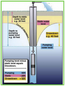
Specific capacity is defined as the rate of discharge of a well per unit depth of drawdown. Expressed as gallons per minute per foot, (liters per minute per meter). It is used as a measure of well efficiency. The ideal for a well is high discharge and low drawdown.
Problem A: - Using the Cooper and Jacob (1946) approximation of the Theis solution to show that the specific capacity, Q/Sw, of a well can be computed from the following equation:

where Q is constant discharge rate [L3/T], rw is pumped well radius [L], S is storativity [dimensionless], sw is drawdown in the well [L], T is transmissivity [L2/T] and t is time [T].
Problem B: Show that specific capacity is controlled predominantly by transmissivity: a very weak function of time, or storage coefficient… in fact it is very insensitive to the dimensionless grouping 2.25 Tt/rw2S in the logarithmic function in the denominator
Problem C: Assuming the following "typical values"
- T = 30,000 US gal/day/ft
- S = 0.001 (confined) or 0.075 (unconfined)
- rw = 0.5 ft
- t = 1 day
Show transmissivity can be estimated in terms of the specific capacity as follows:
- T = 2000*(Q/sw) confined aquifer
- T = 1500*(Q/sw) unconfined aquifer
where T is transmissivity [US gal/day/ft], Q is constant discharge rate [US gal/min] and sw is drawdown in the pumped well after 1 day [ft].
or in metric system … Q in m3/day and sw in m, and T in m2/day :
- T = 1.385(Q/sw) confined aquifer
- T = 1.042(Q/sw) unconfined aquifer
Problem D - simulate groundwater flow in the following area using MAGNET. (Coming soon!)
Given information:
- water well records with specific capacity measurements
- aquifer thickness
- heads/fluxes from sources/sinks
- Well efficiencies: 75%
MAGNET/Modeling Hints:
- Use 'Synthetic Mode' to set up your flow model ( 'Other Tools' > 'Utilities' > 'Go to Synthetic Case Area'). The default model domain for synthetic mode is identical to the domain depicted in the figure above.
- Use the ‘Distance Display’ capabilities when editing geometric features and/or the ‘Ruler’ tool to properly represent distances between model features.
- Conceptualize the model as 1-layer aquifer.
- Use the parameters given input data parameterize your flow model.